Product · CompoundVision

By Compounding Energy

Wind and solar power forecasting for GB, Europe and the US. Hourly, two weeks out. Physics, not black boxes.

CompoundVision produces physics-based power forecasts for 26,300+ wind and solar farms across Great Britain, the EU and the USA (~988 GW nameplate) — and any custom assets you add. Hourly forecasts out to 16 days. The engine is pure physics: Monin-Obukhov atmospheric stability, manufacturer power curves, Perez irradiance transposition, and 30+ documented steps from weather to watts. The physics is never a black box. Probabilistic P10–P90 bands that widen honestly when data is uncertain.

Launch CompoundVision View pricing

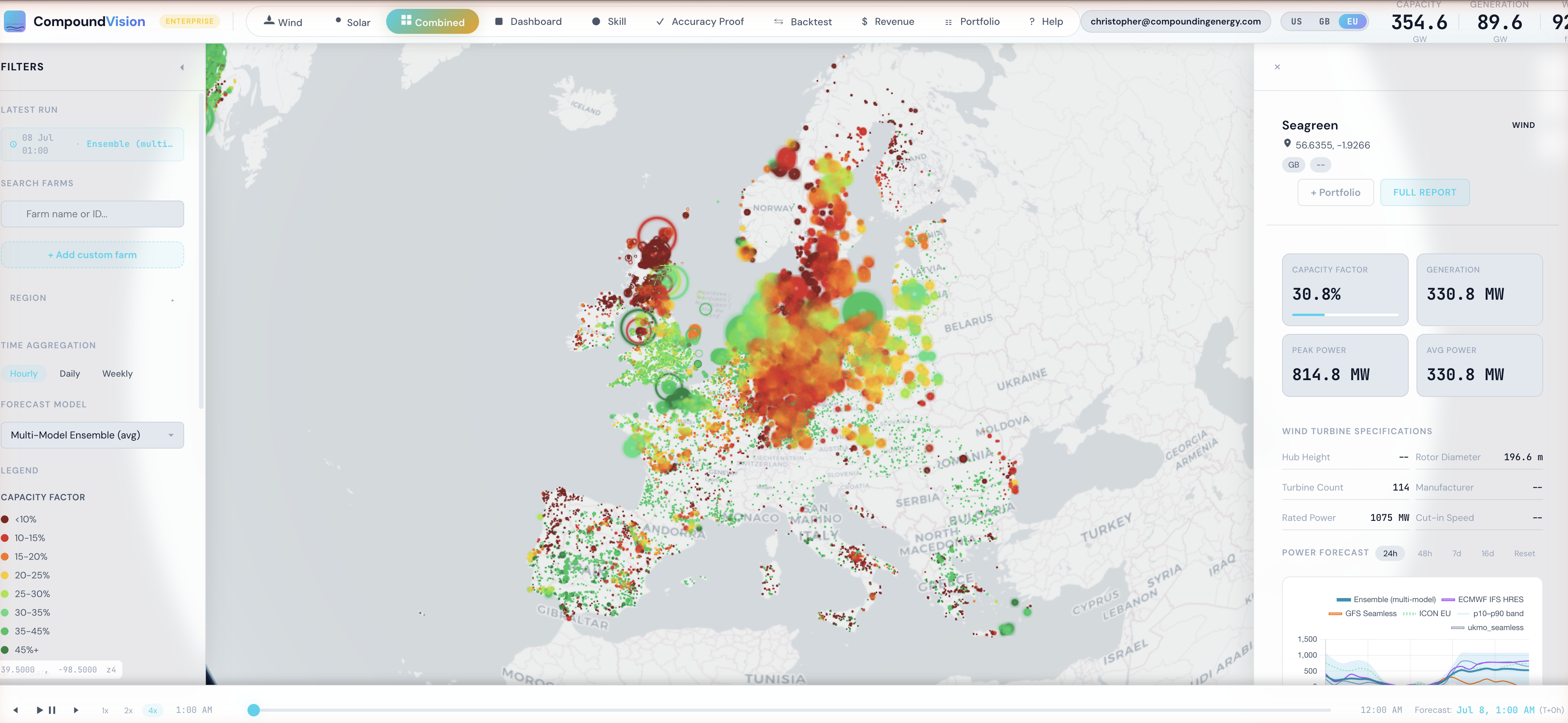
CompoundVision — wind and solar fleet on the 3D globe

26,300+

Wind and solar farms across GB, the EU and the USA — ~988 GW nameplate, each forecast individually from its own specs

16 days

Hourly forecast horizon — every farm, every model, out to two weeks

5 + 2

Five deterministic models — a multi-model average blended from ECMWF IFS HRES, GFS Seamless, ICON Seamless and GEM Seamless — plus two probabilistic ensembles (GEFS 31-member, ECMWF ENS 51-member) for native p10–p90 fan charts.

Revenue

Day-ahead price × power = $ revenue, per hub and per farm, with skill scoring and backtest overlay

How it works

Weather → physics → power → revenue.

Step 1

Weather ingest

CompoundVision pulls hourly NWP data from a multi-model stack — ECMWF IFS HRES, NOAA GFS Seamless, ICON Seamless and GEM Seamless, blended into a multi-model ensemble — plus two probabilistic ensembles (GFS 31-member, ECMWF 51-member). The pipeline is built to scale to 15+ models as we bring more online. Each farm gets weather interpolated to its exact coordinates.

Step 2

Physics-based power conversion

One unified engine runs both wind and solar. Wind: stability-dependent log-law shear (Monin-Obukhov with Louis 1979 closure), humidity-corrected air density, 35+ manufacturer power curves, Bastankhah-Gaussian wake losses, composite curtailment (icing, thermal, high-wind hysteresis). Solar: PSA solar position, Perez 1990 transposition, Fresnel IAM, Faiman thermal model, spectral correction, HSU soiling with rain-wash, bifacial rear irradiance, inverter clipping.

Step 3

Probabilistic output + revenue

Every forecast includes P10, P25, P50, P75, and P90 bands. When a farm's specifications are inferred from vintage defaults (rather than known from the manufacturer), the bands widen by up to 1.4× — so the uncertainty is honest about what it doesn't know. Power multiplies against day-ahead prices to produce $ revenue per hub and per farm. Everything aggregates on a 3D CesiumJS globe or via the REST API.

What you can do with it

Score it, value it, build a portfolio.

Forecasting is the engine; these are the tools desks actually live in — measure how good the forecast is, turn it into money, and combine farms into a book.

Skill & backtest

Know exactly how good it is.

Nightly RMSE, MAE and skill-score against realised generation, broken down by model, region and lead time — so you can pick the right model per market. The Backtest viewer replays any archived forecast over the observed generation for the same window, side by side.

Revenue

Turn power into money.

Forecast power × day-ahead price becomes £/€/$ revenue, per hub and per individual farm, refreshed through the day. Pair it with Skill and Backtest to see how projected revenue tracked what the asset actually earned.

Portfolio

Build and diversify a book.

Group farms into named portfolios, toggle assets on and off, and read aggregated power, per-model comparison, pairwise correlation and variability-reduction σ — so you can see the diversification benefit of adding a site before you commit. Export as portfolio-summary CSV, per-farm CSV, or full JSON.

Physics first, ML where it earns it

When a forecast is wrong, you can trace exactly why.

The power conversion is pure physics — wind speed, air density, atmospheric stability, panel temperature, irradiance geometry. When a farm changes, you update its specs and the forecast adapts immediately. No retraining, no drift, no opaque failure mode. We never use a black box to decide how much power a turbine makes.

A self-learning ML layer sits around that physics core, not inside it. Its job is strictly bounded: fill missing or late-arriving input data, and correct systematic forecast bias a site shows against its own realised generation. The physics stays the source of truth; ML only cleans the inputs and trims known, measured bias.

CompoundVision uses 30+ documented physical steps from raw NWP weather to final power output. Every step is individually testable and physically interpretable. When a forecast is wrong, you can trace exactly why — which atmospheric layer, which power-curve segment, which curtailment rule — and fix it at the source.

Because the ML layer is confined to data-gap filling and bias correction, it can never silently override the physics. You always see the physics forecast and the correction separately.

CompoundVision — per-farm power forecast, multi-model spread and p10–p90 band

Capabilities

Every layer of the platform.

3D CesiumJS dashboard with 9 views

Wind, Solar, Combined, Dashboard (ISO aggregates), Skill, Backtest, Revenue, Portfolio, and an in-app searchable Help manual. Interactive globe with CartoDB basemap, wind particle animation, time scrubber with 1×/2×/4× playback, and marker sizing by capacity, capacity factor, or live power output.

Planned plants + Scenario selector

See the next few years of the grid today. Planned additions carry expected online dates; outlined markers distinguish planned / under-construction / testing from operating, and a Scenario toggle lets you forecast Operating only, + Under Construction, or + All Planned.

Day-ahead revenue

Forecast power × day-ahead price becomes $ revenue per hub and per individual farm, refreshed through the day. Pair it with the Skill and Backtest views to see how revenue tracked against realised generation.

Skill scoring + Backtest overlay

Nightly RMSE / MAE / skill-score vs realised generation — EIA-930 in the US, ENTSO-E and Elexon in GB & Europe — across every model × region × lookback window. The Backtest viewer overlays any archived forecast against the observed generation for the same period.

Portfolio builder with diversification

Build named multi-farm portfolios, toggle farms on/off, and see aggregated power, per-model comparison, pairwise correlation, and variability-reduction σ. Export as Portfolio Summary CSV, Per-Farm Detail CSV, or Full JSON.

Customer farm extensibility

Add your own wind and solar assets via the API or the dashboard's 'Add farm' modal. CompoundVision infers missing specs from vintage-weighted defaults and reports a data-quality badge so you know what's measured vs estimated.

Multi-tenant API

FastAPI backend with JWT + API key auth, per-tenant farm scoping, paginated endpoints for farms and forecasts, and a public tenant that every Explore-tier user can read from. Rate-limited via Redis in production.

Authoritative asset data — GB, Europe & US

In the US, USGS USWTDB and USPVDB are authoritative for operating wind and solar, with EIA Form 860 (annual) gap-filling and 860M (monthly, automated) keeping operating deltas and planned additions current. GB and European farms come from official national and pan-European asset registries. All merged into one unified physics run per cycle.

CompoundVision — ISO-level aggregates dashboard

Companion stack

CompoundVision + CEGridSight

CEGridSight forecasts GB and European electricity prices, generation, and carbon intensity. CompoundVision forecasts wind and solar generation from the physics up — GB and Europe first, the US on top. Together they represent Compounding Energy's approach: transparent, auditable forecasting grounded in first principles.

See CEGridSight View pricing

Research

The thinking behind it.

CompoundVision follows a methodology note from our working-paper series. Shared by invitation while the library is in private beta — request access to read it.

CE-NOTE-2025-03 Working paper Access on request

Training equals production: why we never train on synthetic hindcasts.

The model-serving discipline behind the ML bias-correction layer — training on the same shadows the model serves, never on reconstructions.

Request access